fm_sine_generator

fm_sine_generator(xmod, fs, fc, k, spl_level, print_info=False)

Creates a frequency-modulated (FM) signal of level ‘spl_level’ (in dB SPL) with sinusoidal carrier of frequency ‘fc’, arbitrary modulating signal ‘xm’, frequency sensitivity ‘k’, and sampling frequency ‘fs’. The FM signal length is the same as the length of ‘xm’.

Parameters:

• xmod (array) – Modulating signal, dim(N)

• fs (float) – Sampling frequency, in [Hz].

• fc (float) – Carrier frequency, in [Hz]. Must be less than ‘fs/2’.

• k (float) – Frequency sensitivity of the modulator.

• spl_level (float) – Sound Pressure Level [dB ref 20 uPa RMS] of the modulated signal.

• print_info (bool, optional) – If True, the maximum frequency deviation and modulation index are printed. Default is False

Returns:

• y_fm (numpy.array) – Frequency-modulated signal with sine carrier, dim(N) in [Pa].

• inst_freq (numpy.array) – Instantaneaous frequency, dim(N)

• max_freq_deviation (float) – Maximum frequency deviation [Hz]

• FM_modulation_index (float) – Modulation index

Warning

spl_level must be provided in dB, ref=2e-5 Pa.

See also

am_sine_generator

Amplitude modulation with sine wave carrier

am_noise_generator

Amplitude modulation with broadband noise carrier

sine_wave_generator

Sine wave generation

Notes

The frequency sensitivity ‘k’ is equal to the frequency deviation in Hz away from ‘fc’ per unit amplitude of the modulating signal ‘xmod’.

Examples

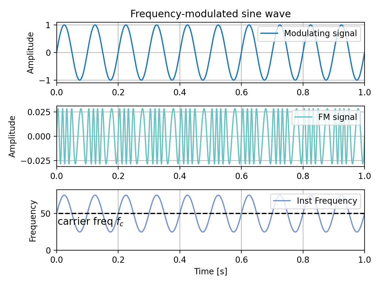
>>> from mosqito.utils import fm_sine_generator
>>> import matplotlib.pyplot as plt
>>> fs = 48000     # [Hz]
>>> duration = 1
>>> t = np.linspace(0, duration, int(fs*duration))
>>> dB = 60        # [dB SPL]
>>> fc = 50        # [Hz]
>>> k = fc//2      # [Hz per unit amplitude of 'xm']
>>> fm = 10        # [Hz]
>>> xmod = np.sin(2*np.pi*t*fm)
>>> y_fm, inst_freq, f_delta, m  = fm_sine_generator(xmod, fs, fc, k, dB, True)
>>> fig, plots = plt.subplots(3, 1)
>>> plots[0].set_title('Frequency-modulated sine wave')
>>> plots[0].plot(t, xmod, 'C0', label='Modulating signal')
>>> plots[0].legend(loc='upper right')
>>> plots[0].grid()
>>> plots[0].set_ylabel('Amplitude')
>>> plots[0].set_xlim([0, duration])
>>> plots[1].plot(t, y_fm, '#69c3c5', label='FM signal')
>>> plots[1].legend(loc='upper right')
>>> plots[1].grid()
>>> plots[1].set_ylabel('Amplitude')
>>> plots[1].set_xlim([0, duration])
>>> plots[2].plot(t, inst_freq, '#7894cf', label='Inst Frequency')
>>> plots[2].legend(loc='upper right')
>>> plots[2].grid()
>>> plots[2].hlines(fc, -0.1, 1.2*duration, color='k', linestyle='--')
>>> plots[2].text(0.0025, fc*0.7, 'carrier freq $f_c$', fontsize=12)
>>> plots[2].set_ylim([0, 1.1*(fc+k)])
>>> plots[2].set_xlim([0, duration])
>>> plots[2].set_ylabel('Frequency')
>>> plots[2].set_xlabel('Time [s]')
>>> plt.tight_layout()

(Source code, png, hires.png, pdf)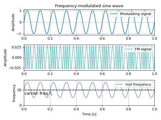