am_noise_generator

am_noise_generator(xmod, spl_level, print_m=False)

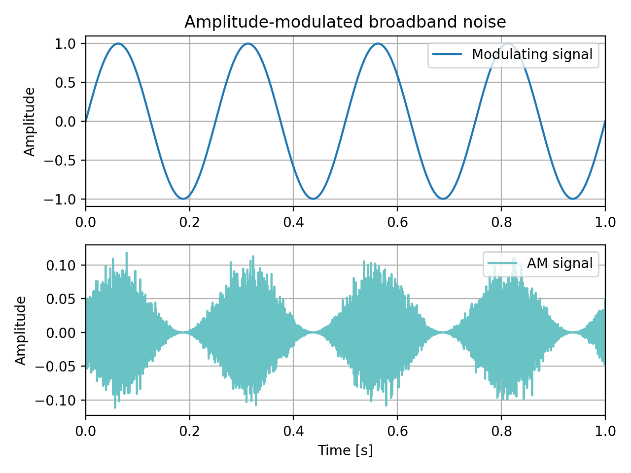
Amplitude-modulated braodband noise generation

This function creates an amplitude-modulated (AM) signal with Gaussian broadband (noise) carrier and arbitrary modulating signal ‘xmod’. The AM signal length is the same as the length of ‘xmod’. The signal level is adjusted to ‘spl_level’ in dB.

Parameters:

• xmod (array) – Modulating signal, dim(N).

• spl_level (float) – Sound Pressure Level [dB ref 20 uPa RMS] of the modulated signal.

• print_m (bool, optional) – If True, calculated modulation index is printed. If False, the modulation index is printed only in case of overmodulation (m>1) Default is False.

Returns:

• y_am (numpy.array) – Amplitude-modulated noise signal in Pascals, dim(N).

• m (float) – Modulation index

Warning

spl_level must be provided in dB, ref=2e-5 Pa.

See also

am_sine_generator

Amplitude modulation with sine wave carrier

fm_sine_generator

Frequency modulation with sine wave carrier

sine_wave_generator

Sine wave generation

Notes

The modulation index ‘m’ will be equal to the peak value of the modulating signal ‘mod_signal’. Its value can be printed by setting the optional flag ‘print_m’ to True.

For ‘m’ = 0.5, the carrier amplitude varies by 50% above and below its unmodulated level. For ‘m’ = 1.0, it varies by 100%. With 100% modulation the wave amplitude sometimes reaches zero, and this represents full modulation. Increasing the modulating signal beyond that point is known as overmodulation.

Examples

>>> from mosqito.utils import am_noise_generator
>>> import matplotlib.pyplot as plt
>>> import numpy as np
>>> fs = 48000
>>> duration = 1
>>> t = np.linspace(0, duration, int(duration*fs))
>>> dB = 60
>>> fm = 4
>>> xmod = np.sin(2*np.pi*t*fm)
>>> y_am, MI = am_noise_generator(xmod, dB, True)
>>> fig, plots = plt.subplots(2, 1)
>>> plots[0].set_title('Amplitude-modulated broadband noise')
>>> plots[0].plot(t, xmod, 'C0', label='Modulating signal')
>>> plots[0].legend(loc='upper right')
>>> plots[0].grid()
>>> plots[0].set_ylabel('Amplitude')
>>> plots[0].set_xlim([0, duration])
>>> plots[1].plot(t, y_am, '#69c3c5', label='AM signal')
>>> plots[1].legend(loc='upper right')
>>> plots[1].grid()
>>> plots[1].set_ylabel('Amplitude')
>>> plots[1].set_xlim([0, duration])
>>> plots[1].set_xlabel('Time [s]')
>>> fig.set_tight_layout('tight')

(Source code, png, hires.png, pdf)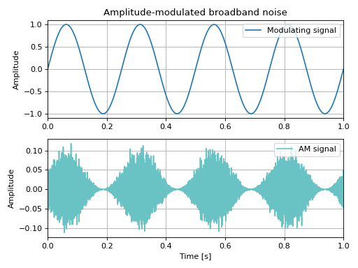